Getting started
Contents
Using JazzHands
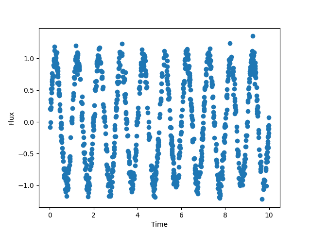
Let’s go through a basic usage example with some synthetic data. First, we’re going to generate a sin wave with a frequency one 1 and amplitude of 1, randomly sampled over 10 periods, with some Gaussian noise added in:
>>> from jazzhands import *

>>> import numpy as np

>>> t_obs = np.random.uniform(low=0.0,high=10,size=1000) #Generate synthetic data

>>> t_obs.sort()

>>> f_obs = np.sin(2*np.pi*1.0*t_obs) #Sin wave with frequency of 1

>>> f_obs += 0.1*np.random.randn(len(f_obs)) #Add in some Gaussian noise
Let’s plot to see how it looks:
>>> from matplotlib import pyplot as plt

>>> plt.scatter(t_obs, f_obs)

>>> plt.xlabel('Time')

>>> plt.ylabel('Flux')
Now let’s initialize a WaveletTransformer object with our data:
>>> wt = WaveletTransformer(t_obs, f_obs)
We now have everything we need to compute a wavelet transform. If you know much about wavelet transforms, you can specify the grid of frequencies/scales, but for now, we’ll assume you just want a quick wavlet transform:
>>> nus, taus, wwz, wwa = wt.auto_compute(nu_min=0.5, nu_max=1.5)
Because real data may have signals at a variety of frequencies, we needed to
specify the window in frequency we want to focus on to improve computational
efficiency. nu_min is the minimum frequency, and nu_max is the max. The
resulting quantities are the frequencies and centers of the wavelets that were
automatically determined when we called auto_compute, the Weighted Wavelet
Z-transform (equivalent to the wavelet power), and the Weighted Wavelet
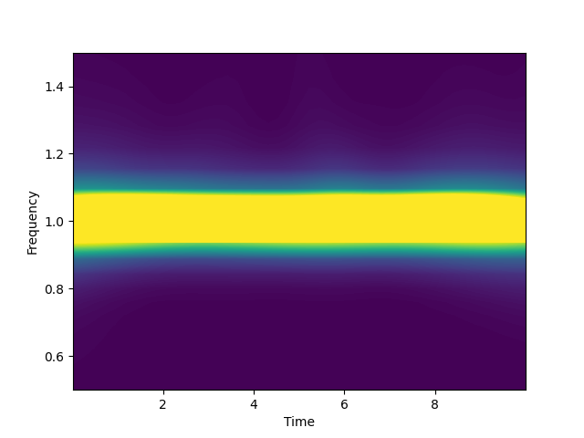
Amplitude. The WaveletTransformer is now populated with some handy attributes
for visualization:
>>> import matplotlib.pyplot as plt

>>> plt.contourf(wt.taus, wt.nus, wwz, levels=1000, vmin=0, vmax=1000)

>>> plt.xlabel('Time')

>>> plt.xlabel('Frequency')
Customizing the Transform
Now that you’ve run the wavelet transform, let’s see what options are built in.
The conventions for the wavelet scale/frequency/dilation are many and varied.
We use three: the frequency (nu), the angular frequency (omega, or 2 pi nu),
and the scale (1/nu). If you know which frequencies/scales are you want, you
can specify either when initializing the WaveletTransformer
>>> taus = [0,0.5,1.0,2.3,4.7]

>>> scales = [0.7,1.0,1.1,1.3]

>>> wt = WaveletTransformer(t_obs, f_obs, scales=scales, taus=taus)
or later, by explicitly setting variables before running compute_wavelet:
>>> wt = WaveletTransformer(t_obs, f_obs)

>>> wt.taus = taus

>>> wt.scales = scales

>>> wwz, wwa = wt.compute_wavelet()
You can also change the decay constant of the wavelet envelope using the c
parameter when initializing the WaveletTransformer; c is set to 0.0125
(approximately 1/8pi) by default, and as long as it’s less than 0.02, you
shouldn’t run into too much trouble. c dictates the tradeoff between time
and frequency resolution as a function of frequency. The
WaveletTransformer.resolution method lets us check these if we supply a
frequency:
>>> wt = WaveletTransformer(t_obs, f_obs, c=0.0125)

>>> print(wt.resolution(1.0))

>>> wt_2 = WaveletTransformer(t_obs, f_obs, c=0.00625) #setting c to 1/16pi

>>> print(wt_2.resolution(1.0))